
Abstract
This article focuses on the solar panel defect detection algorithm – the multi-scale YOLOv8-MNS algorithm. Firstly, it elaborates on the research background, including the importance of solar panel defect detection in the context of the “dual-carbon” goal and the problems in existing detection methods. Then, it comprehensively introduces the YOLOv8 model and the three major improvement strategies of the proposed algorithm: the improved C2f module C2f-MS, the addition of NWD to the loss function, and the replacement of NMS with Soft-NMS. Through detailed simulation experiments and result analysis, it is verified that the improved algorithm has better performance in terms of accuracy, parameter amount, and computational complexity. Finally, the article concludes that the algorithm has certain application value and prospects, and also points out the limitations and future research directions.

1. Introduction
1.1 Research Background and Significance
In the context of the global pursuit of “carbon peaking in 2030 and carbon neutrality in 2060”, solar energy, as an important renewable energy source, has received extensive attention. China’s solar photovoltaic power generation industry is developing rapidly. By the end of 2021, the cumulative grid-connected installed capacity of photovoltaic power generation in China has reached approximately 305.9870GW. Solar panels, as the core component of photovoltaic power generation systems, their quality and performance directly affect the power generation efficiency and service life of the entire system.
However, in the actual production and use process, solar panels are prone to various defects due to manufacturing processes, environmental factors, and human factors. Common defects include cracks, fragments, scratches, and broken grids. These defects not only reduce the power generation efficiency of solar panels but may also cause safety hazards. Therefore, accurate and efficient detection of solar panel defects is of great significance for ensuring the stable operation of photovoltaic power generation systems, improving energy utilization efficiency, and reducing maintenance costs.
1.2 Research Status of Solar Panel Defect Detection
Traditional solar panel defect detection methods mainly include visual inspection, infrared imaging, and electroluminescence imaging. These methods have certain limitations, such as low detection accuracy, high labor intensity, and poor real-time performance. With the development of computer vision and deep learning technology, automated defect detection methods based on machine vision and deep learning have gradually become the mainstream.
Deep learning target detection models are mainly divided into two categories: one-stage algorithms such as the YOLO series directly predict the target frame and category; two-stage algorithms such as Faster-RCNN first generate candidate regions and then perform classification and regression. Many scholars have applied different deep learning models to solar panel defect detection and achieved certain results. For example, the literature proposes a multi-scale photovoltaic panel defect detection method that combines attention mechanisms, which effectively realizes the detection of photovoltaic panel defects. The YOLO series has also been widely studied in solar panel defect detection. For instance, the literature uses the YOLOv3 model to detect defects in solar panel electroluminescence images and optimizes the prior box through K-means clustering to achieve relatively accurate detection. The literature proposes an improved YOLOv5 network structure, introducing the Ghost Module to reduce the number of network model parameters, and simultaneously introducing the SE attention mechanism and the Bidirectional Feature Pyramid Network (BIFPN) to improve the model’s detection performance.
1.3 Problems in Existing Detection Methods and the Purpose of This Research
Although the existing deep learning-based solar panel defect detection algorithms have achieved good detection results, there are still some problems. For example, for small targets in solar panel defects, there is relatively little research, and many models have large volumes, which are not conducive to the deployment of practical applications, indirectly increasing the cost of practical applications.
Therefore, this article aims to study the problems of insufficient detection ability for small targets and large model parameters and computational complexity in solar panel defect detection. By proposing an improved YOLOv8 model, the detection accuracy of the model is improved, and the number of parameters and computational complexity are reduced, so that it has better practical application value.
2. YOLOv8 Model Introduction and Algorithm Improvement
2.1 YOLOv8 Model Structure Overview
The YOLOv8 algorithm is the latest version of the YOLO target detection algorithm series. Its network structure consists of three parts: the backbone feature extraction network (Backbone), the feature fusion network (Neck), and the detection head (Head). These three parts work together to achieve efficient target detection functions.
The backbone feature extraction network is composed of Conv, SPPF, and C2f modules. The C2f module combines the design ideas of the C3 module in YOLOv5 and the ELAN module in YOLOv7, obtaining richer gradient flow information under the premise of lightweight. The feature fusion network is composed of Upsample, Concat, and C2f, mainly performing feature fusion to integrate multi-scale feature information and provide more comprehensive feature expressions for subsequent target detection tasks. The detection head adopts the mainstream decoupled head structure, separating the classification and detection heads. At the same time, it uses an Anchor-Free model, directly predicting the center point and width-height ratio of the target instead of predicting the position and size of the Anchor box. This method can reduce the number of Anchor boxes, accelerate non-maximum suppression, and improve detection speed and accuracy.
2.2 Improvement of the C2f Module
2.2.1 Construction of the MSConv Module
The MSConv module is constructed based on the ideas of depthwise separable convolution and scale-aware modulation (SAM). Depthwise separable convolution consists of channel-wise convolution and point-wise convolution. Channel-wise convolution performs convolution feature extraction operations on each channel of the feature map independently, and then point-wise convolution (1×1 convolution) is used to fuse the features of each channel. SAM includes two key parts: MHMC (Multi-Head Mixed Convolution) and SAA (Scale-Aware Aggregation). MHMC introduces depthwise separable convolution with different convolution kernel sizes to capture spatial features at multiple scales. By increasing the number of heads, the receptive field can be expanded, and the ability to model long-distance dependencies can be enhanced. SAA is a lightweight aggregation module that reorganizes and groups the features of different granularities generated by MHMC and then uses 1×1 convolution for cross-group information fusion within and between groups to achieve a lightweight and efficient aggregation effect.
In the MSConv module, half of the input channels do not perform convolution operations, one-fourth of the channels perform 3×3 convolution, and the other one-fourth perform 5×5 convolution. Then, the feature maps of different scales under various independent channels are concatenated in the channel dimension, and finally, a 1×1 convolution operation is performed to adjust the number of channels. This convolution can capture different details and scale information of the input feature map by using convolution kernels of different sizes, improving the model’s perception ability of multi-scale features. At the same time, by separating the channels of the input feature map, redundant multiplication operations are avoided, reducing the computational complexity.
2.2.2 Replacement of the C2f Structure with C2f-MS
In this article, the MSConv module is used to replace part of the Conv in the C2f module, and the improved C2f-MS structure is used to replace the C2f structure with a channel number greater than 512 in the original model. Through the use of different-sized convolution kernels, the C2f-MS structure can capture different details and scale information of the input feature map, enhancing the model’s perception ability of multi-scale features and improving the model’s expression ability. At the same time, the C2f-MS structure effectively reduces the computational complexity and computational overhead of the model.
2.3 NWD Loss Function
2.3.1 IoU and Its Limitations
The Intersection over Union (IoU) is a commonly used metric to evaluate the performance of target detection algorithms. It measures the overlap degree between the detection result and the ground truth annotation. In the target detection task, the algorithm outputs a series of bounding boxes to represent the detected target position, and IoU calculates the ratio of the intersection area to the union area of the algorithm output bounding box and the ground truth bounding box to measure their similarity.
However, the IoU metric has certain limitations. For small target labels in the solar panel defect data set, due to the small number of pixels and discrete changes in scale, a small positional deviation can lead to a significant decrease in the IoU value. And the IoU metric is very sensitive to the positional deviation of small target labels and has great differences in sensitivity to different scale targets.
2.3.2 NWD Principle and Advantages
The Normalized Gaussian Wasserstein Distance (NWD) is a normalized Gaussian distance metric based on the Wasserstein distance. In target detection, it is used to measure the similarity between the predicted bounding box and the ground truth target bounding box. NWD models the bounding box as a two-dimensional Gaussian distribution, calculates the distance between them, and uses a normalization operation to reduce the influence of factors such as size and spacing.
The calculation method of NWD is based on modeling the predicted bounding box and the ground truth target bounding box as two-dimensional Gaussian distributions. Through modeling, the bounding box can be represented as a Gaussian distribution with a mean and a covariance matrix. Then, NWD uses the Wasserstein distance between these two Gaussian distributions to measure their similarity. The formula for calculating the Wasserstein distance is:
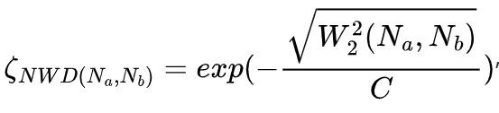
where C is a constant closely related to the data set, and W2^2(Nα,Nb) is a weight parameter used to measure the relationship between the real box loss and the predicted box loss.
Compared with IoU, the Wasserstein distance used in NWD can measure the similarity of distributions regardless of whether the targets overlap. And NWD is insensitive to targets of different scales and combines the Wasserstein distance and the normalization operation of the target, considering factors such as the position, size, and confidence of the target and normalizing them to reduce the influence of the target size and spacing. Therefore, NWD is more suitable for measuring the similarity between small targets.
2.3.3 Integration of NWD into the Loss Function
In the solar panel defect data set used in this article, some targets in the labels are small, and it is easy to miss detections during the detection process. However, considering that not all labels are small and the convergence speed of using NWD is slower than that of the original CIoU, only the NWD loss is added to the original model’s loss function to improve the ability to detect small targets. While improving the ability to detect small targets, the original CIoU loss is still retained, and the convergence speed will not be greatly affected.
2.4 Soft-NMS Non-Maximum Suppression
2.4.1 Problems with Traditional NMS
The Non-Maximum Suppression (NMS) is a post-processing module in the target detection framework, mainly used to delete highly redundant target boxes and only retain the box with the highest score of the same category within a certain area. The process of NMS is as follows: first, select the prediction bounding box B1 with the highest confidence from all candidate boxes as the reference, and then remove all other bounding boxes whose IoU with B1 exceeds a predetermined threshold. Then, select the bounding box B2 with the second-highest confidence from all candidate boxes as a reference and remove all other bounding boxes whose IoU with B2 exceeds the predetermined threshold. Repeat the above operations until all prediction boxes have been used as references, and at this time, no two bounding boxes are too similar.
However, for NMS, in the scene of dense targets, the detection boxes of two targets may have a high IoU. If the detection box with a higher confidence is directly deleted, it may cause missed detections and reduce the recall rate of the model. Moreover, NMS uses the confidence score as the measure of prediction accuracy, but in some cases, the prediction box with a higher confidence score is not necessarily more accurate.
2.4.2 Soft-NMS Principle and Improvement
For Soft-NMS, during the NMS process, for the detection targets with high IoU overlap with the high-confidence target, instead of directly deleting them, the confidence score is reduced. This makes these targets have the opportunity to be retained as correct detection boxes later, avoiding false detections of targets. At the same time, when reducing the target score, a guiding principle is that the larger the IoU between a detection box and a high-confidence detection box, the greater the decrease in its confidence. The Gaussian confidence reduction strategy is:
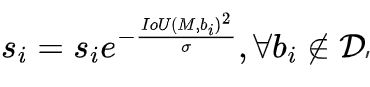
where si is the confidence score of the i-th box, M is the high-confidence box, bi is the other boxes, and σ is a parameter.
Soft-NMS is suitable for solving the problem of missed detections caused by directly deleting highly overlapping targets in the NMS process in dense detection scenarios. This article uses Soft-NMS to replace the NMS in the original model. Soft-NMS retains more candidate boxes, which helps to capture some small targets, occluded targets, or dense targets that are easily overlooked. This can improve the detection recall rate, reduce missed detections and false detections in the case of target aggregation, and also solve the problem of multiple detection boxes appearing for the same target, further improving the detection results.
3. Simulation Experiment and Result Analysis
3.1 Experimental Environment Configuration
The experimental environment configuration in this study is as follows: the CPU uses Intel(R) Xeon(R) CPU E5 – 2686 v4, the graphics card is 3070 Ti – 8G, the CUDA version is 11.7.0, the system is Ubuntu 20.04.5 LTS, the PyTorch version is 1.13.1, the CUDA version is 11.7.0, the Python version is 3.8.0, the initial learning rate lr0 is set to 0.01, the momentum is 0.937, the optimizer is Adamw, the IoU is 0.7, the batch size is 32, the number of workers is 8, and the image size is 640×640.
3.2 Evaluation Criteria and Data Set
3.2.1 Evaluation Criteria
The evaluation criteria in this article include the number of parameters (Parameters), the amount of computation (GFLOPs), mAP@0.5 (the average mAP with an IoU threshold greater than 0.5), mAP@[0.5:0.95] (the mAP under multiple IoU thresholds), and FPS. mAP@0.5 reflects the change trend of the model’s precision with the recall rate. The higher the value of this index, the easier it is for the model to maintain a high precision at a high recall rate. mAP@[0.5:0.95] represents the mAP under multiple IoU thresholds. In the interval [0.5, 0.95], with a step size of 0.05, 10 IoU thresholds are taken, and the mAP under these 10 IoU thresholds is calculated respectively, and then the average value is taken. The larger the mAP@[0.5:0.95], the more accurate the prediction box is, because it takes into account more cases with large IoU thresholds.
3.2.2 Data Set
The data set used in this article is obtained from the PP PaddlePaddle (AI Studio), including 600 solar panel defect images, which are labeled and expanded to 2400 images through flipping and rotation. These images are divided into a training set of 1920 images and a validation set of 480 images according to a ratio of 4:1. The entire data set contains three types of defects: scratches, broken grids, and dirt. The defect images of the three types are shown in the following table:
| Defect Type | Image |
|---|---|
| Scratch | [Image of Scratch] |
| Broken Grid | [Image of Broken Grid] |
| Dirt | [Image of Dirt] |
3.3 Experiment on the Improved C2f
To ensure the fairness and significance of the improvement and avoid possible biases or interferences, no pre-trained models were loaded before and after the improvement. To verify the adaptability of the improved C2f-MS structure to the entire model, experiments were conducted by replacing the C2f in different positions with C2f-MS. The experimental results are shown in the following table. The experimental types are as follows: Type 1 replaces the C2f structure with a channel number greater than 512 in the entire model; Type 2 replaces the C2f structure with a channel number less than 512 in the entire model; Type 3 replaces all C2f structures in the entire model. Experiments were also conducted on the convolution of different convolution kernels in 1/4 of the channels in MSConv for different experimental types.
| Convolution Kernel Number | Experimental Type 1 (mAP@0.5/mAP@[0.5:0.95]) | Experimental Type 2 (mAP@0.5/mAP@[0.5:0.95]) | Experimental Type 3 (mAP@0.5/mAP@[0.5:0.95]) |
|---|---|---|---|
| 1,3 | 0.886/0.458 | 0.857/0.443 | 0.853/0.432 |
| 1,5 | 0.881/0.454 | 0.87/0.443 | 0.88/0.443 |
| 1,7 | 0.882/0.447 | 0.872/0.447 | 0.861/0.435 |
| 3,5 | 0.887/0.453 | 0.882/0.454 | 0.871/0.452 |
| 3,7 | 0.866/0.446 | 0.871/0.446 | 0.87/0.445 |
| 5,7 | 0.882/0.448 | 0.868/0.447 | 0.882/0.459 |
It can be seen from the experimental results in the table that when the convolution kernel number is [3,5] and the C2f structure with a channel number greater than 512 in the entire model is replaced, the mAP@0.5 is the highest; when the convolution kernel number is [5,7] and all C2f structures in the entire model are replaced, the mAP@[0.5:0.95] is the highest. From the above experimental data, it can be seen that the overall effect of Experimental Type 1 is better than that of the other two experimental types, and when the convolution kernel number is [3,5] and the improved C2f structure is used to replace the C2f structure with a channel number greater than 512 in the entire model, the overall index is better. Therefore, subsequent improvement experiments will be carried out on this basis.
3.4 Ablation Experiment
In this article, the network model is improved through three improvement schemes. To explore the impact of the three improvement schemes on the research results, an ablation experiment is carried out on the improvement points. The specific experimental data are shown in the following table. The three improvements are as follows: replacing the C2f structure with a channel number greater than 512 with the improved C2f-MS structure, adding NWD to the original loss function CIOU, and replacing the NMS in the original model with Soft-NMS.
| C2f-MS | NWD | Soft-NMS | Parameters/10^6 | GFLOPs | mAP@50/% | mAP@[0.5:0.95]% | FPS |
|---|---|---|---|---|---|---|---|
| x | x | x | 3 | 8.2 | 87 | 45.7 | 76.34 |
| √ | x | x | 2.7 | 7.7 | 88.7 | 45.3 | 66.67 |
| x | √ | x | 3 | 8.2 | 88 | 45.5 | 76.34 |
| x | x | √ | 3 | 8.2 | 88.8 | 49.2 | 67.11 |
| √ | √ | x | 2.7 | 7.7 | 89 | 46.1 | 64.94 |
| √ | √ | √ | 2.7 | 7.7 | 89.5 | 49.8 | 59.88 |
It can be seen from the above data that when only one improvement is used, the mAP@50 of the model can be improved, and the overall performance of the model can be improved. However, when only C2f-MS and NWD are used, although the mAP@50 is improved, the mAP@[0.5:0.95] is slightly decreased. When only Soft-NMS is used, compared with the other two improvements, the mAP@50 and mAP@[0.5:0.95] are improved the most, with an increase of 1.8% and 3.5% respectively. Soft-NMS reduces the confidence between candidate boxes to reduce overlapping detection results, thereby reducing missed detections and false detections in the case of target aggregation. The combination of the three improvements obtains the greatest benefit. Compared with the original model, the number of parameters of the improved overall algorithm is reduced by 9.57%, and the amount of computation is reduced by 6.1%. When the number of parameters and the amount of computation are both reduced, the mAP@50 is increased by 2.5%, from the original 87% to 89.5%; the mAP@[0.5:0.95] is increased by 4.1%, from the original 45.7% to 49.8%. In summary, the improved model not only has lower parameters and computational complexity than the original model, but also has higher detection accuracy. The improved model shows better detection performance in the experimental results.
3.5 Comparative Experiment and Detection Effect
To objectively analyze and compare the performance of different methods in solar panel defect detection, this article compares and analyzes the proposed algorithm with the algorithms in the literature [6], YOLOv3, YOLOv5, and YOLOv7 in terms of the number of parameters, the amount of computation, and mAP. The experimental results are shown in the following table.
| Model | Parameters/10^6 | GFLOPs | mAP@50/% | mAP@[0.5:0.95]% |
|---|---|---|---|---|
| Literature [6] | 49.6 | 299.3 | 76.2 | 41.3 |
| YOLOv3 | 103.7 | 283.0 | 89.3 | 47.9 |
| YOLOv3 – Tiny | 12.1 | 19.0 | 86.9 | 43.5 |
| YOLOv5s | 9.1 | 24.0 | 86.9 | 45.5 |
| YOLOv7 | 37.2 | 105.1 | 86.5 | 43.6 |
| YOLOv7 – Tiny | 6.0 | 13.2 | 80.4 | 38.3 |
| This Article | 2.7 | 7.7 | 89.5 | 49.8 |
It can be seen from the data in the table that the algorithm in this article has the highest mAP@50 and mAP@[0.5:0.95] among all the models. The mAP@50 is 13.3 percentage points higher than that in the literature , and the mAP@[0.5:0.95] is 11.5 percentage points higher than that of YOLOv7 – Tiny. In terms of the number of parameters and the amount of computation, the improved algorithm in this article is lower than any algorithm in the comparative experiment. The number of parameters is only 2.6% of that of YOLOv3, and the amount of computation is only 2.57% of that in the literature. In summary, the algorithm in this article not only has better accuracy than the algorithms in the comparison, but also has a relatively lightweight number of parameters and computational complexity, showing better detection performance in solar panel defect detection and being more conducive to practical deployment.
To more intuitively and efficiently show the detection effect of the algorithm in this article, the detection images before and after the improvement are shown in the following figure.
According to the figure, it shows the detection effects of the original label, the original model YOLOv8n, the algorithm in this article, and some other algorithms. By comparing the detection effects of different algorithms, the following three conclusions can be obtained:
(1) The original model has the phenomenon of false detections. The improved model enhances the ability of multi-scale feature extraction and fusion, effectively avoiding the occurrence of some false detections.
(2) The confidence value of the improved model is higher than that of the original model.
(3) For the scratch defect, the original model has multiple detection boxes at the same label, and the detection result of the improved model avoids the appearance of multiple detection boxes. Overall, the improved model improves the detection accuracy, reduces the probability of false detections, and avoids the situation of multiple detection boxes at the same label.
4. Conclusion
In this article, an improved YOLOv8 model for solar panel defect detection is proposed. By using the C2f-MS structure, the number of model parameters and computational complexity are reduced, and the ability of multi-scale feature extraction and fusion is enhanced. Then, NWD is used to optimize the original loss function to improve the detection performance of small targets and balance the detection ability. Finally, Soft-NMS is used to replace the original NMS to solve the problem of multiple detection boxes for the same target. The experimental results show that the overall detection performance of the improved YOLOv8 model is improved, and the number of parameters and computational complexity are also reduced, making it more convenient for deployment on mobile devices.
However, due to the limitations of experiments and data sets, only three types of defects, namely scratches, broken grids, and dirt, are studied in the experiment, and other defects are not studied. In future research, more defects will be studied to further optimize the defect detection performance of the relevant algorithm. It is expected that with the continuous development of technology and the expansion of research scope, the performance of solar panel defect detection algorithms will be further improved, providing more powerful technical support for the development of the solar energy industry.